The Frequency Inside the Noise

Close your eyes. Listen to a piano playing a single key. Simple, clean, one thing.

Now listen to a full chord. Now someone talking. Now static from a broken radio.

Here is what a physicist notices: none of those sounds are different in kind. They are all the same thing — air pressure wiggling your eardrum. The difference is not in what is happening. It is in the story happening underneath — how many rhythms are layered on top of each other, and at what speeds.

Learn it once for sound, and your brain will automatically speak the same vocabulary for every wave system you ever meet: water, light, rotating fluids, even the slow inertial sloshing of a lake responding to a storm.

The Simplest Possible Thing: A Mass on a Spring

Before complexity, we need to understand simplicity. Pull a mass away from its resting position. The spring fights back with force $F = -kx$. Newton takes over:

The solution is a perfect, eternal cosine:

One number, $\omega_0$ — the natural frequency — tells the whole story. Stiffer spring, faster rhythm. Heavier mass, slower rhythm. The system has a preference, one particular beat it falls into whenever you disturb it.

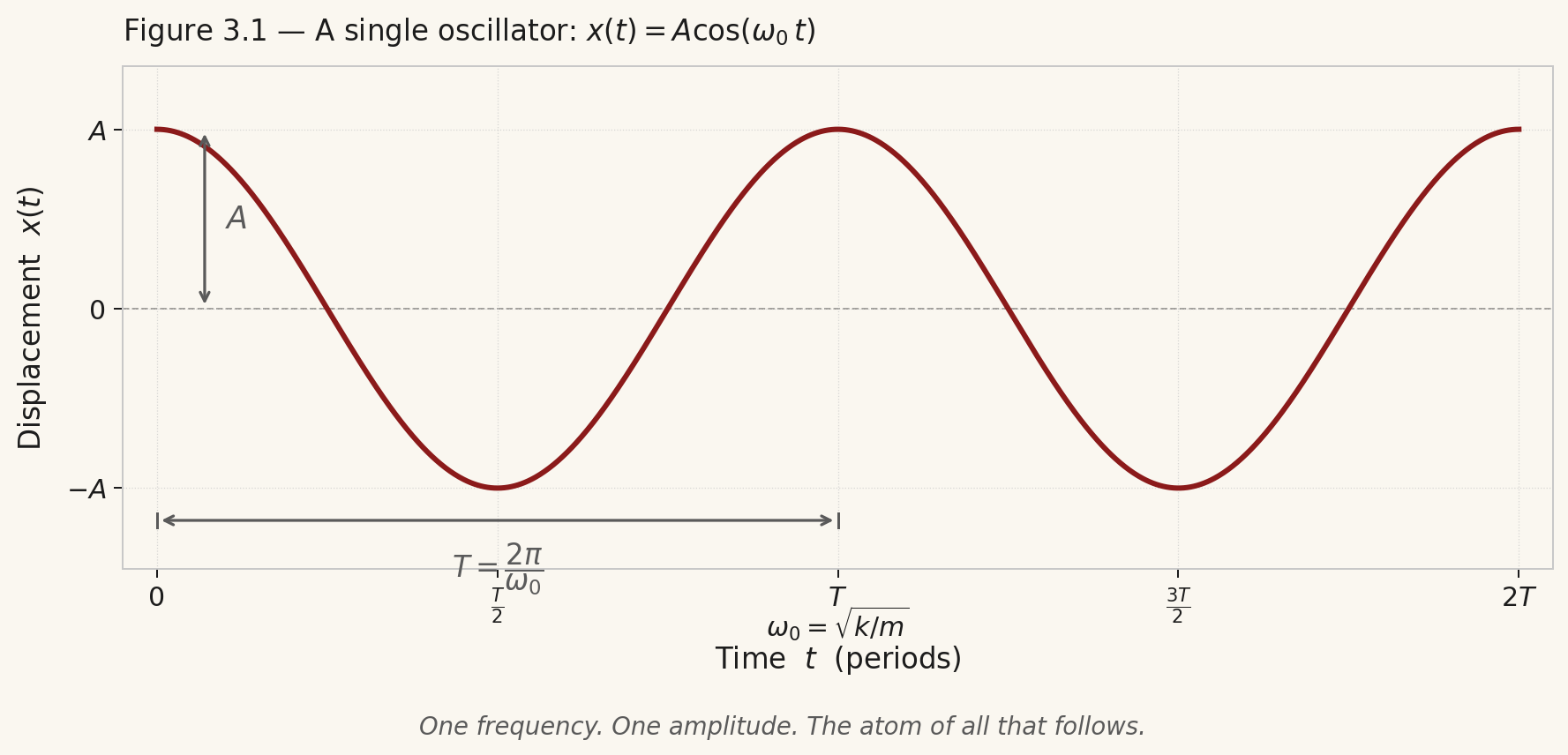
Hold this picture in your mind. It is the atom of everything that follows.

Sound: The Best Classroom Nature Ever Built

A Pure Tone Is a Spring Wearing an Acoustic Costume

Sound is air pressure doing exactly what the mass on the spring does. A tuning fork at 440 Hz pushes and pulls air molecules, which push their neighbours, and a pressure wave travels outward. At your eardrum:

One frequency. One pure tone. One Fourier component. This is the note A above middle C, and a tuning fork sounds like a tuning fork precisely because it produces almost nothing else — no other rhythms hiding underneath.

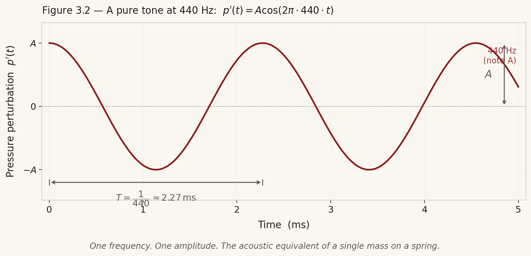
Now ask: what does this look like not in time, but in frequency? If you mapped "how much of each frequency is present," you'd get a single spike at 440 Hz. Dead silence everywhere else. That right there — that map — is the beginning of the Fourier transform.

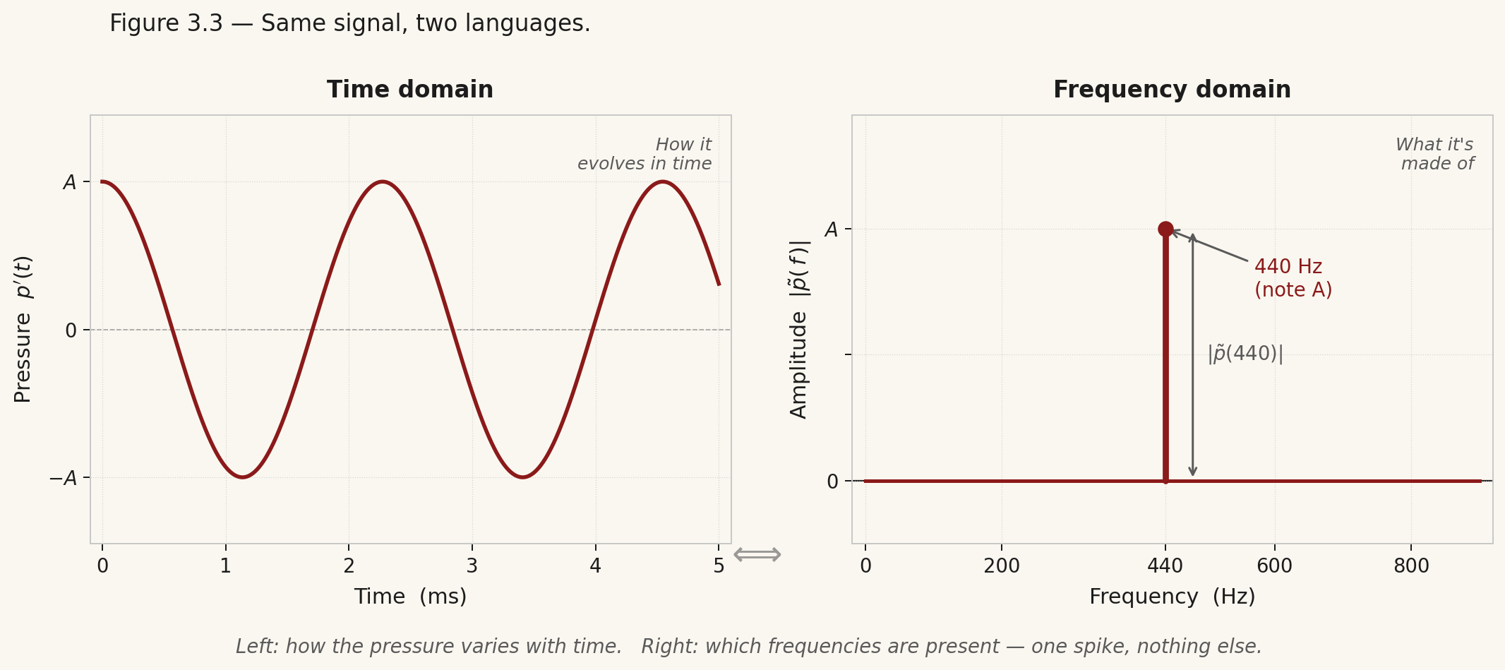
Same signal. Two languages. The left panel tells you how it moves through time. The right panel tells you what it is made of.

A Chord — Where the Story Gets Interesting

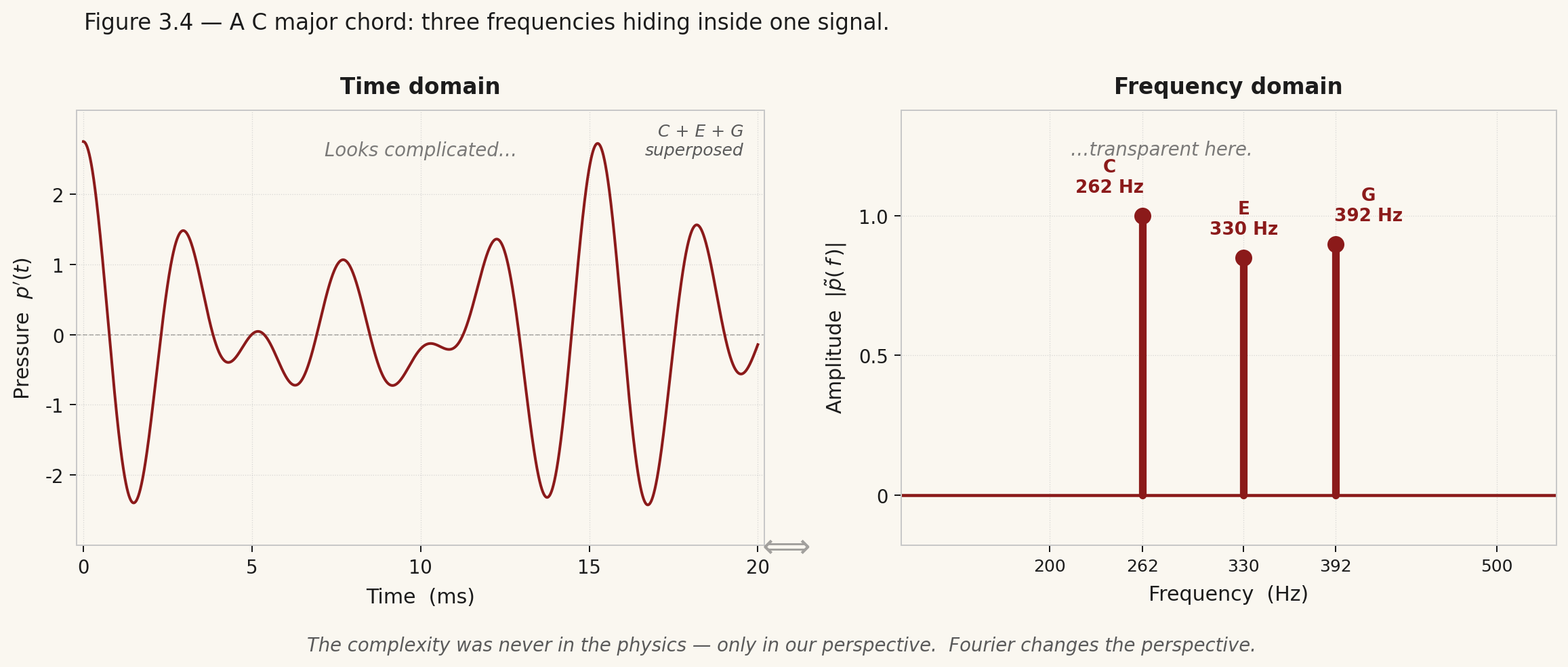
Press C (262 Hz), E (330 Hz), and G (392 Hz) at once. A C major chord. The pressure at your eardrum is now three cosines, stacked:

The time-domain signal looks like a mess — nothing like a clean cosine. But the frequency-domain picture? Three clean spikes. C, E, G. The structure never disappeared. It was just hiding.

The Human Voice — Where It Gets Wild

A spoken vowel — say "ah" — is not three frequencies. It is hundreds. Your vocal cords vibrate at a fundamental pitch, maybe 150 Hz, and the shape of your throat and mouth amplifies certain harmonics — multiples of that fundamental — while damping others. Those amplified clusters are called formants, and they are precisely what makes your voice sound like yours and not like anyone else's, even on the same note.

Look at the time-domain waveform of a spoken vowel: crumpled paper. Look at the frequency spectrum: a harmonic ladder rising from the fundamental, with two formant humps draped over it like a tent. Completely readable. The vocabulary of the voice, written in frequency.

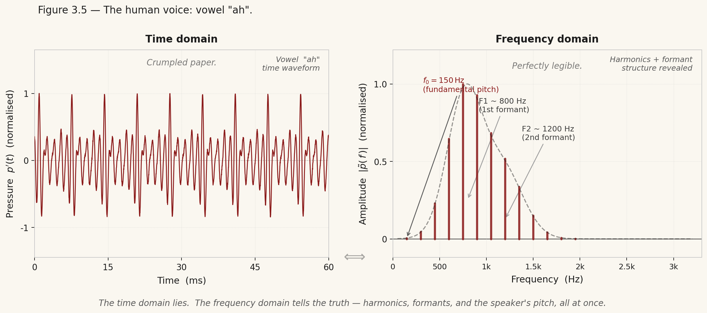
The information was always there. The transform just taught us to read it.

Your Ear Has Been Doing This Since Before You Were Born

Here is the part that stops students cold: you do not need a computer to perform Fourier analysis on sound. You are doing it right now, physically, inside your skull.

The cochlea — the spiral-shaped organ of your inner ear — is lined with roughly 16,000 hair cells. Each one is tuned to a different frequency. High frequencies fire cells near the base of the spiral. Low frequencies fire cells near the tip. When sound enters, different cells respond in proportion to how much of their particular frequency is present in the signal.

Your cochlea is a biological Fourier spectrum analyser. The fact that you can pick a friend's voice out of a noisy room, or tell a violin from a piano on the same note — that is real-time Fourier decomposition, running in wetware, continuously, without you doing a thing.

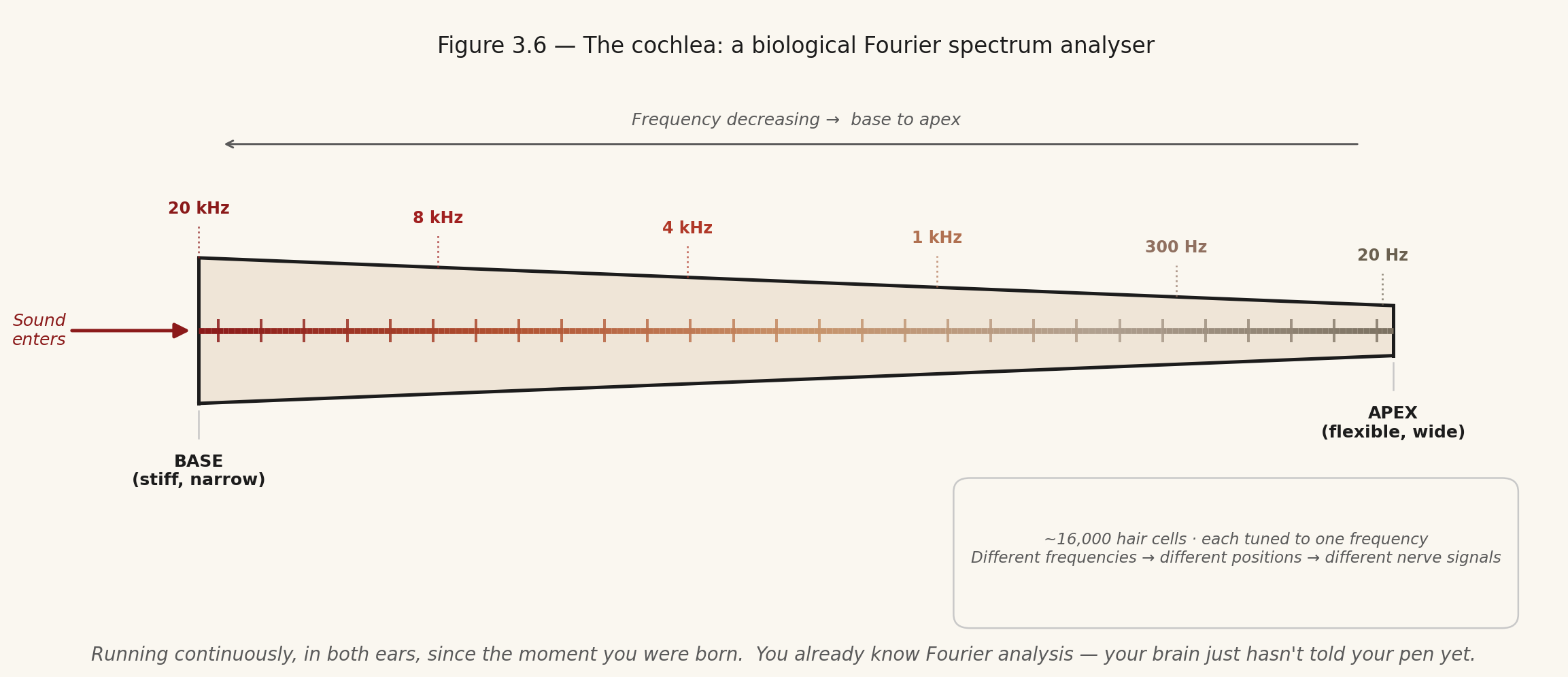
If your brain already understands Fourier analysis, the mathematics is just your pen catching up to what your ears already know.

What Is Fourier Analysis?

Joseph Fourier was a French mathematician who, in 1822, published one of the most quietly revolutionary ideas in the history of science. His claim: that any signal — no matter how complicated, no matter how irregular — can be written exactly as a sum of pure sine and cosine waves, each with its own frequency and amplitude. Not approximately. Exactly. The great Lagrange rejected it at first. Fourier was right.

Think about what that means for a moment. You record the sound of a thunderstorm. Chaotic, violent, seemingly structureless. Fourier says: hiding inside that chaos is a clean, exact list of frequencies — each one a pure tone, each with a definite loudness. Find the list, and you understand the storm. That is the promise of Fourier analysis, and it keeps its promise every single time.

The mathematical tool that finds that list is the Fourier transform:

Do not let the integral intimidate you — it is asking one simple question, once for every possible frequency $\omega$: how much of this frequency is hiding inside the signal $f(t)$? The term $e^{-i\omega t}$ is a probe — it oscillates at frequency $\omega$, and when you multiply it against $f(t)$ and integrate over all time, you get a large number if $f(t)$ vibrates strongly at that frequency, and nearly zero if it does not. Run this for every $\omega$, and you have the full inventory — every rhythm present in the data, and how loudly each one is speaking.

To get back from frequency to time, you run the inverse:

This says: rebuild $f(t)$ by adding up all the pure oscillations, each weighted by how much of it is present. Together, these two equations form a transform pair — a lossless, exact, reversible translation between two equally complete descriptions of the same reality. Not a single bit of information is created or destroyed. You are not approximating anything. You are simply changing the language.

In practice, the quantity physicists reach for is the power spectrum:

Real. Non-negative. Directly readable. It tells you how much energy the signal carries at each frequency. A sharp peak means the system has a natural mode there — it loves to oscillate at that rhythm. A broad smeared peak means the same mode exists but is damped, bleeding energy fast. A flat, featureless spectrum means pure random noise — no preferred frequency, no hidden structure, nothing to read.

Here is a small, concrete example. Drop a stone into still water. The ripples spread outward. In the time domain, you see a complicated undulating surface, rising and falling, impossible to read by eye. In the frequency domain, you see something clean: the energy is concentrated at the frequencies dictated by the depth of the water and the size of the disturbance. The chaos in the time domain was never fundamental — it was just many simple waves, all talking at once. Fourier analysis is how you hear each voice separately.

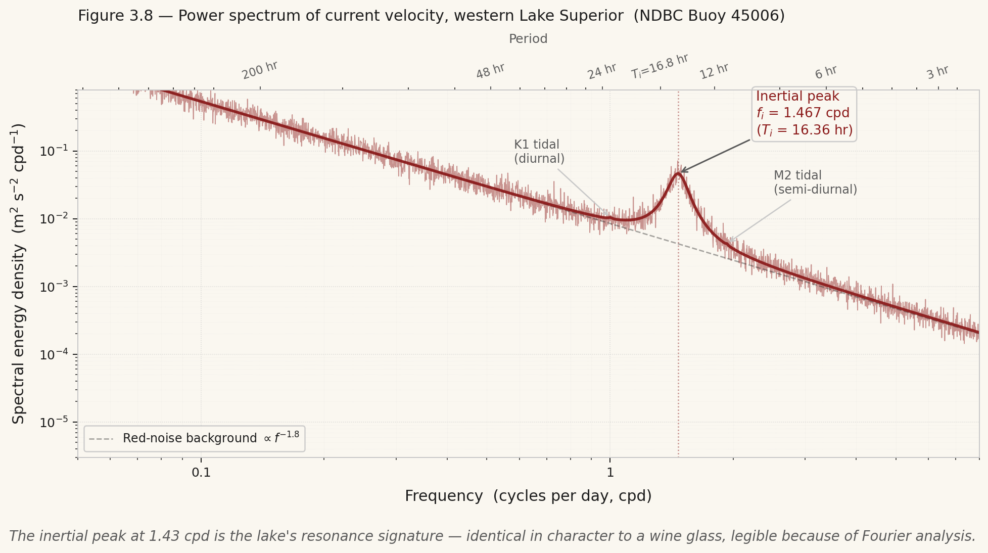
Applied to Lake Superior: years of raw current velocity measurements look like nothing but noise in the time domain — a jagged, restless, seemingly structureless record. Transform that record into the frequency domain and a sharp peak appears at exactly 1.43 cycles per day, corresponding to a period of 16.8 hours. That is the inertial frequency — the rhythm the lake falls into every time a storm disturbs it, the fingerprint of the Earth's own rotation encoded in the motion of the water. The Fourier transform did not add that information. It was always there. The transform simply made it readable.

Making It Exact: The Transform

It Is a Change of Vocabulary, Not a New Subject

You already know how to decompose a vector:

Each component tells you how much of each direction is present. The basis vectors are orthogonal — they do not talk to each other — so the decomposition is clean and unique.

A signal $f(t)$ is the same thing, but in an infinite-dimensional space. The Fourier transform decomposes it onto a basis of pure oscillations $e^{i\omega t}$. These are also orthogonal — a sine at 440 Hz does not contaminate a sine at 441 Hz. The decomposition is still clean, still unique.

The forward transform is a probe: for each frequency $\omega$, it asks how strongly does this signal vibrate here? The integral accumulates the answer over all time. Large result means lots of that frequency. Near-zero means it is absent.

And these two equations are not approximations. Not a single bit of information is lost. Time domain and frequency domain are the same story told in two different languages.

The Power Spectrum — The Diagnostic Tool You Will Actually Use

Physicists do not usually work with $\tilde{f}(\omega)$ directly — it is complex-valued, which makes it harder to read at a glance. Instead, we reach for the power spectrum:

Real. Non-negative. And physically clear: it tells you how much energy the signal carries at each frequency. This is what your audio equaliser displays. What a seismologist reads after an earthquake. What we compute from ocean current records.

Here is the thinking pattern — the diagnostic story — that works for any signal you ever encounter:

Memorize the logic of that story. The formulas follow naturally once the logic is in your bones.

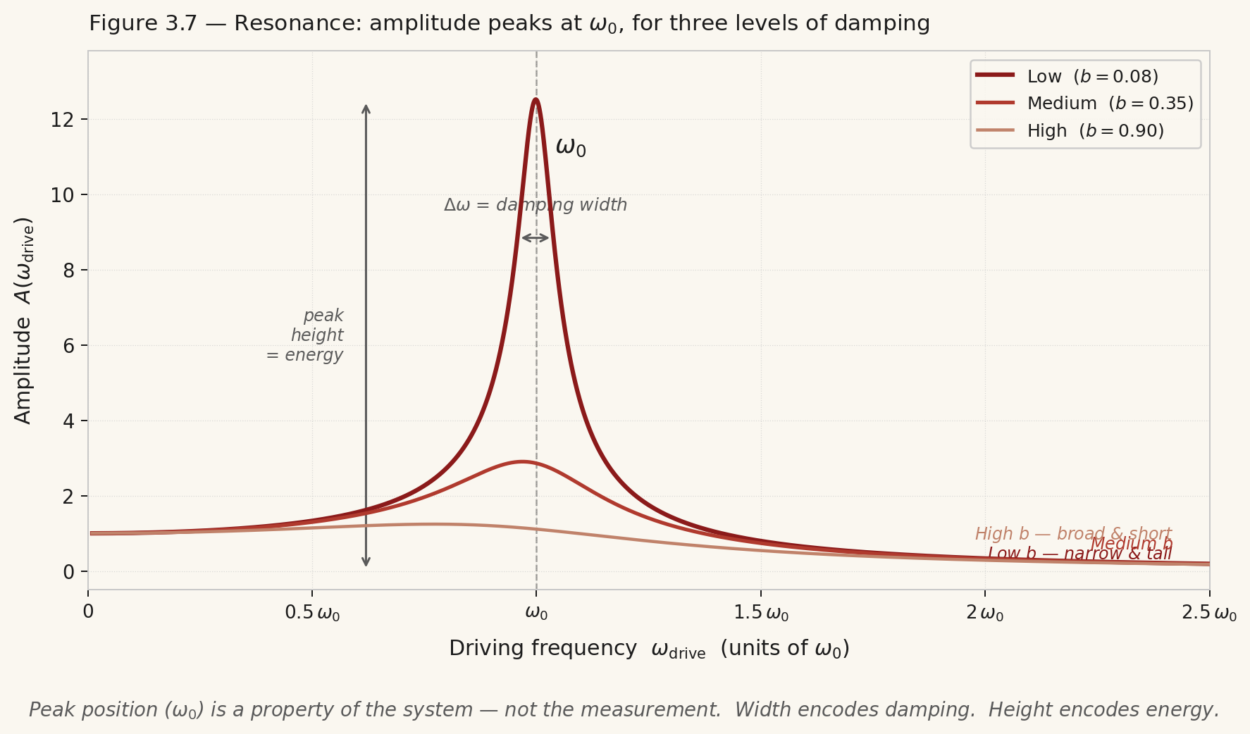
Resonance — When a System Has Strong Opinions

Every oscillating system has a natural frequency, and it has a strong preference for it. Drive it at that frequency and energy accumulates — the amplitude grows, sometimes violently. This is resonance, and the power spectrum is how you find it without waiting for something to break.

Add driving and friction to the oscillator:

The steady-state amplitude is:

Peak at $\omega_{\text{drive}} = \omega_0$. In the power spectrum, this shows up as a Lorentzian — a peak with a specific shape. Its position is always $\omega_0$, a property of the system, not of how you measured it. Its width encodes damping. Its height encodes energy.

A wine glass has a natural frequency. Sing that note loudly enough and the glass shatters. A soprano knows this intuitively. A physicist reads it in the spectrum before the glass breaks.

The Seven-Step Vocabulary — Your Portable Toolkit

Every time you encounter a wave, an oscillation, a fluctuating signal of any kind — run this story through your head.

Seven steps. Works on sound, light, ocean waves, gravitational ripples in spacetime. Fourier is not a technique. It is a way of reading the universe's handwriting.

The Leap: From a Concert Hall to a Lake

You have seen that a sound wave in air obeys:

Now look at the equation governing velocity in a rotating fluid — the kind of wave that sloshes in a lake when a storm passes overhead:

Look at the structure. The Coriolis parameter $f$ — the Earth's rotation rate projected onto the local vertical — is playing the role of the spring constant. The fluid velocity $u$ is the mass. The system has a natural frequency: $f$ itself, the inertial frequency.

Disturb a rotating fluid — a storm, a pressure front — and even after the forcing stops, the fluid keeps oscillating at $f$. These are near-inertial oscillations, and they show up as a peak in the power spectrum of current measurements, at frequency $f/2\pi$, exactly as a piano string's resonance shows up as a peak in its acoustic spectrum.

Lake Superior sits at roughly 47°N. The Coriolis parameter there gives an inertial period of approximately 16.8 hours. A current meter moored in the western basin, recording velocity over years, shows that peak standing clear above the background — the lake's resonance signature, the fingerprint of the Earth's rotation encoded in the motion of the water.

One Technical Reality You Cannot Ignore

In practice, you never have an infinite continuous signal. You have $N$ measurements, spaced $\Delta t$ apart. Two hard limits follow immediately.

The Nyquist limit: You cannot see frequencies higher than $f_{\max} = 1/(2\Delta t)$. Anything above that folds back into the spectrum as a ghost frequency — an alias — and corrupts what you are reading. Sample fast enough, or filter first.

Frequency resolution: With total record length $T = N\Delta t$, the finest frequency difference you can resolve is $\Delta f = 1/T$. Wanting to separate the inertial peak from a nearby tidal line? You need long records — weeks to months of data.

These are not bookkeeping details. They are physical constraints on what is knowable from a finite window of observation. Every audio engineer, every oceanographer, every seismologist lives inside these same walls.